Table of Contents
Do you like to color-code your cells? Most of us do it. It makes it easy to understand what’s going on with just a glance. When you have a lot of data listed all the way down to the bottom of a spreadsheet, it can be pretty daunting. Thankfully for us, Google Sheets (or any spreadsheets for that matter) gives us the option to go in and change the color of that sheet.
Can Google Sheets automatically color-code cells based on the value that’s found within that cell? The answer is yes. Google has a feature called conditional formating and what that means is that you can create a set of rules and as long as the condition is met, it will automatically format the cell the way you instructed it to. It’s very easy to do and it makes your spreadsheet a powerful tool for analyzing data.
This tutorial is about getting Google Sheets to change the color of a cell automatically based on a rule that we provide it.
Take for example if you happen to record your profits and losses from your business and want an easier way to quickly recognize what’s profiting and what’s losing you money, you can make Google Sheets do it for you.
Let’s say you completed a job and earned $100. For simplicity’s sake, $50 is the profits you’ve gotten from this job. You would label this as a “high profit” in Google Sheets. As you complete more jobs, you begin a long list of profits and unfortunately, losses in your spreadsheet. The reason why you may have losses is perhaps you underestimated the cost of materials and supplies. Or perhaps the client didn’t pay you. You’ve now got 100’s of lines of profits and losses throughout the year and it’s really hard to visually glance through your list to see how well you’ve been doing.
At this point, you might want something a little more visually pleasing when trying to skim through your list. We can automate Google Sheets so that if it sees any value higher than a certain amount or even a word such as “high profit” to make the cell background the color green. And maybe if we only made between $0 to $15, we can simply call it a “low profit” and then make Google designate that as yellow. And God forbid if we lost money, we can instruct Google Sheets to turn cell that has a negative value or the keyword “loss” as red.
Doing so will help improve your perception of how well the business is running. If you saw a column full of green then I’d say you’re business is in great shape. If you see a column with half red and half green, then that might be something you want to go back into and reevaluate. Maybe your operations need a little tweaking. The point of this article is to help you figure out if your business or project is going in the right direction so that you can the modifications to improve it.
Again, the concept is generally known as conditional formatting.
Changing the color of the cells based on values (Easy method)
- Open Google Sheets.
- Highlight the column on your table.
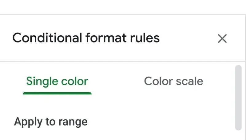
- Go to Format > Conditional formatting.

- Make sure you are in the Single color tab
- Click on Format rules.
- Select the appropriate rule based on the value inside your cells
- Click on Formatting style.
- Make your changes to the way you want your cells to look according to your Format rules.
- Click Done.
- Repeat these steps if you want more conditions.

Changing the color of cells based on custom formula values (More powerful method)
- Open Google Sheets.
- Highlight the column on your table.
- Go to Format > Conditional formatting.
- Make sure you are in the Single color tab
- Click on Format rules.
- Select Custom formula is at the bottom
- Type in the formula with the correct syntax.
- Click on Formatting style.
- Make your changes to the way you want your cells to look according to your Format rules.
- Click Done.
- Repeat these steps if you want more conditions.
Why choose the custom formula option instead of the format rules already created by Google Sheets?
Google Sheet’s template of format rules is easy to use. But at the same time, they are for simple formatting. They won’t help with anything that’s too complicated.
When you choose the custom formula option, you can put in a formula that goes beyond the capabilities of the usual templates you see here.
Try this out. In step 2, highlight a column of your choosing. Follow through the steps above but when you reach step 7, type this in but choose a completely different cell that’s not a part of the highlighted column you chose earlier. Type in =B2=“green” as the custom formula. Make sure the B2 shown above is not a part of your highlighted column. Complete the styling steps and click done.
From now on, if Google Sheets were to see the word “green” in cell B2, it would make the other column that you highlighted the style you chose.
As you can see, this has an indirect effect on one cell that signals the change to another cell. This isn’t something that’s an option in the template format rules. It’s a custom formula and it can be very powerful once you’ve learned more and more of the syntax.
What’s the difference between apply to range and format rules in Google Sheets?
It helps to fully understand the difference in what we are working with within the conditional format.
Range to apply is the cells or the group of cells we want the results to happen to. This is where we set our parameters and boundaries. Usually, you would select the entire data table or even just a row or column within it and if you want a condition to make this green, then that’s what would happen in your range to apply to a group of cells.
Format rules tell Google that this is the test to see if this is a true statement. This part is based on a condition that we create.
If our “Format rules” is true, then it will display the results into our “Range to apply”.
How to make the color change stretch entire rows based on a value
Once again, you can customize how you want the formatting to behave. This can only be done if you’ve selected to create a custom formula.
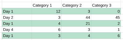
You’ll need to highlight an entire row based on criteria. This can be a little confusing but I’m going to try to walk you through the difference and what this part of the topic is trying to do and why you need it. The image below helps explain it a little clearer. I’ve made the condition where it must highlight the background green every time it sees the word “Day 1.” As you can see, all the Day 1 rows are highlighted.
Why would you want a certain color to stretch an entire row? Well, maybe it’s just for aesthetic reasons, or maybe doing this will help improve the look of the spreadsheet.
You see, spreadsheets can get really large with data tables full of information from one row to another row with columns packed to the brink.
If you create a conditional formula using the method above, you’ll only see that one particular cell highlighted according to the style you chose.
This method allows the entire row to be highlighted in that particular style. For many, this can help improve the way the spreadsheet looks.
Let’s say you have data that is conditionally formatted to green but it’s located at the very right of the spreadsheet. You might have even had to scroll to the right to get there. Now, what if you wanted to see what day that data was entered but the day column requires you to scroll back to the left. How do you align these two pieces of information with your eyes as you scroll further and further away out of sight?
One way to do it is to place your finger on the screen and just scroll back, that way your finger stays in that row position and ends up pointing to the right Date row.
Another way is to make the format highlight the entire row automatically.
In this situation, we need to follow a few rules. The first rule is that the alphanumeric location of the cell that you’re going to use as the location of the condition MUST be located within the table itself. This isn’t like the steps above. It has to be one of the cells located inside the table. Another rule is that this cell must have the criteria you are looking for.
So take for example here. F2 is a cell located inside the table and it has the word “green” in it. That’s the condition we are looking for. If anything else has the word “green” in it and its within the table, we want to highlight the entire row green.
The final rule to make this right is that the cell you are pointing to must be the very first occurrence of that word. It can’t be the second or third because if you point to that second or third, what this does is offsets what Google Sheets will highlight green.
We accomplish this by adding in a dollar sign ($) before F2 which makes it =$F2=”green” to lock-in that value so that it doesn’t move or shift along with every condition test made.
What this will do now is highlight the entire row as long as you previously designated your range to be the entire table.
You must understand the syntax when working on conditional formatting rules
It’s important to understand syntax because if you get this wrong, Google Sheets won’t know what you’re talking about. When you write =B2=”high profit” within the formula text box, you need to know what every symbol, every punctuation, and every word makes a difference.
In Google Sheets, if you are trying to create a formula you must start with an equal sign (=). This signals Google Sheets to expect a formula or a function.
This is where it might get a little confusing. B2 is part of the conditional statement. It needs to match the row or the number of the first row of the range you created above. If I wanted to start my range in C3:C for example, I would have to change my B2 condition statement to C3. If I wanted to start my range from D3:D, it would be appropriate to change my condition to D3. And you can hopefully get the picture with what I’m trying to say here.
Finally, you need to set that cell (ie. the B2, or C3, or D3, whichever you choose) to equal the particular value you’re looking for. In this case, high profit is considered a string and when we deal with strings, we place them within parentheses.
My conditional formula is not working and the range seems shifted in one direction
Going back to the conditional statement location, it can be a bit confusing. I know. I tried testing a few scenarios out making my range start at B2 while making my condition start at B3 and it seems to shift all the results up by one cell. It’s kind of hard to explain but if I modified these values for range B2:B to show yellow with the condition of B3=”profit”, it would test if B3 is true or false. If it were true then it would make the cell above it yellow instead of itself yellow which isn’t what I had intended. It would then continue to test the next row below that so if B4 were true, it would make B3 yellow.
So there seems to be some sort of shifting that goes on here. I can’t explain it really well.
I went further to testing out this theory and it seems to be true. This time I tested the range B2:B with a condition at B4 and it seems this time that all results had shifted up by 2 cells. This time, the yellow showed up 2 cells above the true condition.
The solution I’ve found to this is again from above. The cell that we are testing in the conditional statement must be a cell located within the table and it must test the first occurrence of that condition. So don’t just make the conditional cell a part of the header of the table, just place it in the very first cell that holds data to test it.