Table of Contents
Referring to data from the same file is a simple task. In fact, if you’re interested, I’ve written an article about that here (How to link a single data cell between different Google Sheets).
Can you actually refer to data that’s located in one Google Sheets file and make it show up in another separate Google Sheets file? The answer is yes. In order to do so, there is a specific formula made just for this. The function IMPORTRANGE can be used in a formula along with a URL reference to the spreadsheet and the range will allow you to reference data from one file to another.
This is quite different from simply referring to data from a spreadsheet in the same file. It’s also a bit different from referring data from two different tabs of spreadsheets that are in the same file. We are talking about referring to data that is located in a totally separate Google Sheets file altogether. It’s an important distinction because it really changes what you will need to use and do to make it work properly.
Let’s say, for example, I have a Google Sheet file called “A” and I have another Sheets file called “B.” These are completely different Google Sheet files, not just different spreadsheet tabs within the same file. I want to use data from file A and cross that data over to file B. Well, Google Sheets has a function that allows us to do this.
After some research, I’ve found the solution to this problem. Check out the simplified steps below.
How to reference data from one Google Sheets file to another
In this example, let’s assume you have a Sheet we’ll name “Target” which is the file we want the data to end up in. The other Sheet will be named “Data” which will be where the data is coming from.
- Start on your Target Sheet.
- Select and highlight a cell.
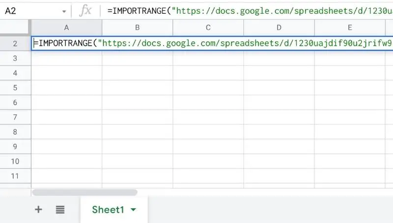
- Type in =IMPORTRANGE(“”,””)
- Go to your Data Sheet and copy and paste the entire URL in between the first set of quotation marks of step 3.
- Determine the range of data from the Data Sheet (ex. A1:F13) and place that range between the second set of quotation marks of step 3.
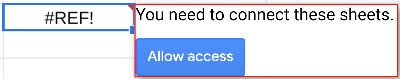
- Hover over the Target Cell (which should say something like #REF!) and tap on Allow access
What Should the Formula Look Like?
=importrange(“https://docs.google.com/spreadsheets/d/1NyxedF39H97dgoG3VYasdfT7j8X3asf30cHKjfjs$6FY/edit#gid=0″,”A1:F13”)
Check out the full syntax from my example. This is purely an example, it doesn’t lead to any data. Your URL and range should be different, but otherwise, it should look very similar to this.
What is =IMPORTRANGE?
What’s happening here is that the function =IMPORTRANGE actually imports data from another spreadsheet file.
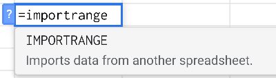
This means that its sole purpose is to take in data that are located one another spreadsheet. You can still do quite a bit with this method but that’s a discussion for another topic.
What is the first quotation marks?
The next part of this formula is the first set of quotation marks which answers the question, from where is this data coming? Where can I find the file that this data is located in?
The answer is to simply copy down the entire URL address of the target sheet and paste it here.
What is the second quotation marks?
The last part of the puzzle tells the formula exactly what data you are looking for within this URL file. It’s looking for an actual alphanumerical location or a range of it. You’d type that location in between the second quotation marks and you’re good to go.
Allowing access is only required once
Luckily for us, allowing access to use the data from another sheet is only required once. If you want to reference from the same Data Sheets again in a different cell of your Target Sheets, you don’t have to again “Allow access”.
Allowing access seems to work globally with a spreadsheet. If I were to add more data into the Data Sheet and then turn around and reference that data to my target sheet, I wouldn’t have to ask for permission access again. Allowing access is only required once.
If the owner of the spreadsheet removes you, then your access is revoked
Also, let’s say that Data Sheets is owned by someone other than you and the file has been shared with you. If for whatever reason, the owner happens to remove you from the shared list, your access to this file will be revoked.
The data you’ve referenced will no longer work and will disappear from your own spreadsheet.
This method will no longer work until the owner shares the file with you again.
My data sheet has multiple tabs, how do you refer to data from specific tabs?
One thing you might be questioning is what happens if the spreadsheet with all your data in it is comprised of multiple tabs? All of with have data in them.
If you’re Data Sheet has multiple tabs, the formula won’t be able to tell which tab to take the data from. There are multiple versions of the range so how is it suppose to choose? The formula will actually still try to guess anyway. In fact, it’s going to automatically default to the very first tab and choose to show whatever range you’ve chosen in that first tab.
So how do you add the name of the tab in an =importrange function? In order to specify the tab within the spreadsheet containing data, you have to add in the tab name, surrounded by single quotes. You do this by placing the tab name (surrounded by single quotes) inside the second quotation marks where you would normally only place the range. Then you follow after the single quote with an exclamation mark (!). Finally, end it with the usual alphanumeric range.
It should now look something like this:
=importrange(“https://docs.google.com/spreadsheets/d/1NyxadF39497dgOG3ViasdfY7j8Y3asd30cDKjfjs$6FY/edit#gid=0″,”’tab_name’!A1:F13″)
Don’t forget the quotation marks!
Without quotation marks, you will get an error. If you hover over the error it will say something like “Formula parse error”.
Be sure you have those quotation marks around both the URL and the range. When using functions and formulas, everything has to be precise. You need to include every bit of information so that the computer knows and fully understands what you are talking about. These are computers and they need detailed instructions in order to function properly.
I’ve had multiple people reach out to me telling me something was wrong with their formula and that it was showing an error. The majority of the issue fell into forgetting to add these single quotation marks.
Don’t forget the Comma
There’s a comma that separates the URL from the range or in other words the first quotations from the second quotations. The comma tells the formula that one argument (which was the URL you input) has ended and to anything after the comma is another argument. This formula expects 2 arguments and so you’ll get an error that will say something like “Wrong number of arguments”.
Again, it’s very important that you have the syntax complete.