
Table of Contents
I am currently in need of organizing my expenses for a side project that I’m working on. I’ve been told by so many people to learn spreadsheets because that’s the tool I’ll need. After doing quite a bit of online research, I’ve found a neat little trick that creates a drop-down list that I can show you.
Can you use Google Sheets to create a list of options in the form of a drop-down list? The answer is yes. Google Sheets offers a tool called Data validation which will allow you to set parameters and restrictions on what types of values a cell will accept. Data validation is basically the idea of a drop-down list that will restrict the user from inputting anything other than what was intended.
A drop-down list will allow you to click on a cell on the spreadsheets and be given the option to choose from a list of selections.
This method is a little bit special because it will allow you to manually add more to the list at any moment in time.
Now there are two different ways, two different methods that I could find of creating a dynamic drop-down list. Both methods have their advantages and disadvantages in which I can’t wait to discuss.
Let’s begin with the first method.
Creating a dynamic drop-down list (The manual, yet powerful way)
- Open up or create a new Google Sheets
- Create a second sheet by clicking on the plus icon on the bottom left of your screen (you are creating a second tab within the same file. Don’t exit the current spreadsheet, just look for the plus sign at the bottom and click on it. You’ll see a new sheet tab populate).
- Choose any column on this second sheet and enter each item in each cell of that column. For example, if I wanted to create a list of pet animals, I’d write in “dog” in one cell, then “cat” underneath, and then “turtle” underneath that until I’ve written down all the pets I’ve wanted.
- Click on Data tab located above
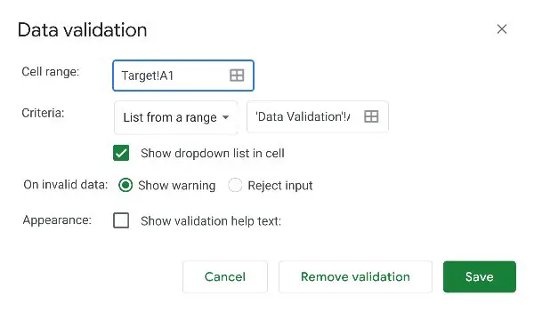
- Look for and click on Data validation

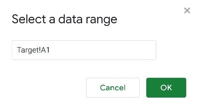
- For Cell range, first, click on the icon to the right of the next box. It looks like 4 boxes, all stacked 2×2 forming a larger box. A new window called Select a data range will show up temporarily replacing the Data validation window.
Then, return to the original sheet (by going to the tab with the specific cell(s) that you want to designate as the drop-down list and select the cell(s) you wish to feature a drop-down list.
Just to be clear, this isn’t the list of pets you’ve just created that’s one on top of the other. If you can still see that list in your background, chances are, you’re on the wrong sheet. This is where you want the user to click and be shown the selection of pets you listed.
If you are curious, the reason it asks for the range is because you can make this drop-down list available for multiple cells on your spreadsheet. This is a helpful tip, for example, if you plan on some type of expense report and for every single time you make a purchase, you can also include a drop-down list for that corresponding purchase.
After you’ve made your cell or range selection, clicking the Ok button should bring you right back to the Data validation window where you will move onto the next step.
By the way, this part is where most of the problems begin. If at any moment after filling out everything and clicking on Save shows a read bar with a warning text. I think I may know why. Scroll down to the subheading titled, “How to fill out Cell range and Criteria correctly.” When you’re done, head back here to continue. - For Criteria next to the textbox to the right of List from a range, once again click the 4 squares that form a larger box and then switch back to the second sheet (the sheets with the list of items in it) and highlight the list of items you’ve created in the column from step 3. If you are having problems with this part, again, I’ve laid it out clearly in the subheading titled, “How to fill out Cell range and Criteria correctly.” Spoiler alert, it’s the syntax you most likely got wrong.
- To make the list dynamic, highlight not only your created list but also a few extra blank cells in that column. If you do continue to highlight more of the blank spaces underneath, then in the future if you want to add to the list, you can simply just go straight to this sheets tab and add it into a selected blank cell. You won’t need to do any of the steps above. Your new item should automatically be an option in your other sheet’s drop-down list the moment you save the spreadsheet
- Click Save
- If any of the steps above are not working right for you, I’d recommend reading further down this article. I’ve compiled a list of issues and key points that I think may help you in how Google Sheets operates regarding drop-down lists.
A few extra Tips you should Know
While learning how to create these drop-down lists, I’ve come across a few things I’ve noticed as a novice that might help you understand how it all works.
You can create multiple sheets within the same Google Sheets file
In Step 2, you need to create another sheet. This may sound weird, but Google spreadsheets allows you to create multiple sheets within the same spreadsheet.
You can perhaps create your list of items on the same sheet that you plan on making the drop-down list, but I wouldn’t recommend it. Keep the sheet clean and keep the listed items separated from the drop-down list.
If you look down at the bottom of Google Sheets, you’ll see a plus sign along with (by default) a tab named “sheet1.” By clicking on the plus symbol, you’ll notice that another tab forms automatically named “sheet2.”
To keep it organized, you can even rename these sheets simply by using your mouse to right-click on that tab and clicking on rename. The second sheet you created is only used to create the items list. You can even name this sheet “Data validation.” You would rarely need to use it again unless you were wanting to add even more items to that list.

When adding each item into each cell on the second sheet, it doesn’t matter if you skip cells but traditionally, you should type them all in, each one below the previous cell.
When creating a Data validation range, just highlight the entire column
When typing this list of items, make sure you keep this list within the same column. Google Sheets does allow you to highlight a square full of columns and rows and that would work just fine with populating your list of items in your drop-down list, but ultimately it might make things harder for you to understand when you look back at this list.
You can create multiple separate lists of items on the same Data validation sheet
The reason I say it may be confusing if you were to highlight an entire group of rows and columns is that Data validation sheets can have multiple separate drop-down list categories.
One column can be a Data validation list of expenses, another can be the income, and another could even be the vendor all on one sheet tab.
It’s best to stay organized and I found it best to just keep them in columns. Just keep it nice and tidy in your second sheet.
The reason you are asked to highlight a few extra blank cells in step 8 is that in step 7, Criteria is given that information and is told to display that in the Cell range of step 6. If there’s nothing in that cell, it won’t show up in the drop-down list. This can restrict you and even be a little time consuming but in the future, if you just so happen to want to add another item down the line, you can do so on the empty cells you’ve marked for Criteria.
Doing so will automatically add that item to the drop-down list without any further Data validation modifications from you.
Also, don’t worry about the extra blank cells you’ve added to the list. Google Sheets is smart enough to know that blank lists are really just placeholders and it won’t show up as blank selection in your drop-down lists.
What’s the difference between Data validation’s Cell range vs. Criteria
The main issue that I’ve encountered was the lingo that was inserted into both Cell range and Criteria. I scratched my head for quite a bit trying to figure out what they both meant specifically and this is what I’ve found.
Cell range points to the actual cell that has the drop-down list. Criteria points to the list of items you’ve created.
How to fill out Cell range and Criteria correctly
Chances are, if you followed the steps I’ve listed above to the ‘T’ and you’re still having problems, then it is most likely due to you not knowing the proper syntax. This is the way Google Sheets wants you to write it out because if you do it any other way, it most certainly won’t understand you
Take notice of how the syntax is in each textbox. Before you even type anything, Google Sheets offers a suggestion of what exactly it is they’re looking for. In Cell range, you’ll notice that it starts off with the name of the sheet (in my case, Target) then an exclamation mark (!) and finally the range of the first cell (ie. A1) to the last cell (ie. A100) separated by a colon (:). But for now, mine looks something like this “Target!A1”. Again this is located in the Cell range aka my target sheet that needs to show the drop-down window.
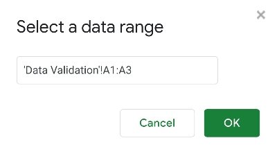
Based on the name you created for your Data validation sheet (the sheet with the list of items you created), you’ll have to do a few modifications to this suggestion as well. Take for example my list. I named my list sheet, “Data validation” and it has a list of 3 items. Inside the A1 cell, I have “dog”, A2 is “cat” and A3 is “turtle”. The proper syntax for me to set inside my Criteria text box would be
Make sure this syntax is written correctly. Without the proper input, your Google Sheets Data validation won’t understand you.
By the way, if you are super detailed oriented and realized that there are single quotes surrounding Data validation within Criteria and not Target within Cell range. Good job! So why use single quotes? The reason for the single quotes is that it’s for sheet names with 2 or more words. If you only have one word, then you don’t need the single quotes. Google will automatically know when it’s just one word, but when it’s two or more, you’ll need to let Google Sheets know that this is the entire name of the sheet tab.
In Criteria, I have “‘Data validation’!A1:A10”. Again, this is the list of items I’ve created plus a few empty cells for future convenience.
Google Sheets Data validation needs to know where it’s getting that data from and the very first part of that syntax is what it looks at.
To recap from what’s above, Cell range is the sheet with the drop-down list. Criteria is the sheet with the list of items.
