Table of Contents
Most people know that there’s a way to easily add numbers to a spreadsheet.
But in case you have never used Google Sheets before or any spreadsheet program for that matter, Google Sheet has the ability to perform functions to a list that you provide it. This list can oftentimes be a set of numbers. All we have to do is tell Google Sheets that we want to find the sum of this list and Google Sheet will automatically add the list up for you.
So can Google Sheets add up the number for you? Google Sheets does have the ability to add your data and give you the sum of those numbers. This has been one of the fundamental features that Google has set into Google Sheet for years now. But how does Google Sheets add numbers for you? The simple answer is that Google Sheets is a spreadsheet program. And like any other program, it uses formulas that are somewhat like codes that perform tasks on data for the user Simply call upon this code and tell Google Sheet what range you want it to sum up and the results should appear automatically. But of course, there are several ways you can get the sum of a group of numbers.
One of those options is a simple tool to find the sum of all the items you’ve listed inside the file. But one common mistake is how someone goes about formatting this setup.
Let’s start with how I find the sum of a list of numbers.
How to add up or take the sum of numbers on Google Sheets
- On the same Google Sheets, click on and highlight the cell you wish the resulting sum to show up on.
- Click on the formula icon tab above that looks like 90 degrees counterclockwise rotated M or a sharp-edged E.
- Look for the word SUM.
- Immediately after, select, drag, and highlight all the numbers in the column you wish to add (assuming that you’ve already entered in all your data or numbers).
- Press Enter on your keyboard.
What happens when you use SUM?
After pressing the enter button on your keyboard, you should see the sum combined and conveniently displayed within the cell you originally highlighted.
The displaying of your results can really be on any cell you choose, so find the best place you want your answer to show up every time. It can even be found on multiple places of your choosing as long as you follow the steps above while highlighting a second or a third cell. It’s also important that you place it in a way where it doesn’t obstruct further data from being placed in. For example, if this data were only half way completed and it took time to physically add in more data, you don’t want the display of the SUM in a cell that will later on down get in the way of that data as it grows into more cells.
However, I want to show you a few extra tips that will improve your spreadsheet and make life way easier for you. Seriously, read on.
How to make Google Sheets automatically update the sum as you add in more data
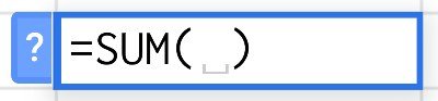
In step 4, take notice as to how you are instructed to drag and highlight all the numbers. You would’ve first seen that highlighted cell populate with the formula
At this point, whatever cell you click on all the way to whatever cell you drag to will be your range. However, simply dragging from one set of data to the last actually limits what we can do in case that set of data is expected to grow bigger and bigger with time. Take for example a Google spreadsheet that you’ve created to record the every expense you make throughout the year. The purchases you make to run and grow your business will continue to occur throughout the year. You wouldn’t happen to write them all down at once at the end of the year. And you really wouldn’t know how many things you need to buy for that year until that year is over.
So how do you prepare your SUM to proactively predict and make room for all your expenses? The answer to that is, instead of limiting to just highlighting the numbers that you currently have filled in, go ahead and highlight several empty cells as well. Those empty cells that happen to be included in the range will not affect the SUM and are available for you to continue to add more and more numbers in the future.
Google Sheet does not recognize empty cells. It won’t be registered and thus the Google will just assume those empty cells are zero (0) in value and that makes no difference when taking a SUM.
Once you add a new number to an empty cell that was previously highlighted int he SUM range, the cell displaying the SUM will automatically update.
People have built entire programs that help spearhead their operations to really high levels when using just this function alone.
How to easily pre-set the entire column in Google Sheets to be SUMed up
If you rather make the entire column add new numbers to your cell that displays the sum, there’s an easy way to do that. The idea is that no matter where you place your data in that designated column, Google Sheet should be able to automatically get the sum of the data right after you’ve added in the data.
Again in step 4, instead of highlighting anything at all and after clicking on the SUM formula from the formula icon, click on the very top cell alphabet. You can see that there are a bunch of alphabetical letters at the top A, B, C, D all enclosed in their own cell.

By clicking on the top lettered alphabet above, you will notice that the entire column is now highlighted. This is exactly what should happen. You’ll also see that the range within the sum formula looks something like =SUM(A1:A999) for example. Or sometimes it may look like this =SUM(A:A), which means the same thing. It means that the formula will calculate all the numbers or data located within the entire column.
Again, don’t worry about all those empty, blank spaces. Google Sheet ignores blank areas.
Place your SUM cell in a spot to avoid overwriting data errors
Now, this part is pretty important in my opinion. I’ve always found myself placing the SUM cell in the wrong position. What’s the wrong position? It’s actually quite common and every novice makes this mistake early on in their spreadsheet career.
Don’t place your SUM cell at the bottom, underneath your the list of data. This is because if you plan to add numbers to be summed up, you’ll eventually run out of space and have to move the SUM cell further down the line.
Of course you wouldn’t do this if you had registered the entire column as a range for SUM like we did in the subtopic above. Placing a SUM cell in the exact same column as the one you designated to hold all your data will pop up with an error. I got error circular dependency detected. My guess is that it tried to add the sum of itself to the SUM result but as it added, its own sum changed… I guess it was looping itself around and that’s where the error came from.
Where should you place the SUM cell in Google Sheets to avoid issues?
I found it most convenient to just place this SUM cell directly above the list of data. That way, as you add numbers to the column (assuming that as you add more data, you add them below the previous data cells), you don’t have to worry about running out of space or colliding with the SUM cell.
Putting the SUM cell at the top is not your ownly option. There’s another great place to put it.
An alternative location is to place the SUM cell on the right side of the column list of numbers. However, if you find yourself adding column categories to that spreadsheet, eventually you’ll collide with this SUM cell as well.
I found that the best approach is to place it right above the data. It’s the first thing you’ll see when you open up the file. Again, this gets the SUM cell out of the way for when your list of data begins to grow.
Modifying your range accordingly when your SUM cell is directly above your list of data
So you’ve decided to place the SUM cell right above the list of data, however, you noticed that after clicking on the entire row, the range of what your taking the sum of is including the SUM cell as well. How do you properly modify the range so that it doesn’t include or get in the way of the SUM in its addition sight?
This is where you have to understand the syntax of the formula. Take a look at the formula below:
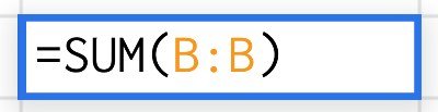
Now, this is what would happen if you were to perhaps click on the alphabet cell above when inputting the range of the SUM formula. The first B to the left is the starting cell and the second B to the right is the final cell. But that doesn’t fully make any sense. They are the same letter. Well, this is the way most if not all spreadsheets understand what it means when taking in an entire column. Alternatively, you can write =SUM(B1:B999), assuming that the last cell in your column is cell number 999. This is the range and everything in between this range is added to the SUM cell. All you have to do is change the first B to point to the very first data in your Sheet. Now oftentimes, you will have subheadings organized or placed right above these lists of data so that it is clear to the reader and even to yourself.
Going back to you owning a small business and having an expense sheet. You’ll want to do something like placing the subtitle Expense right above the list of data. Well, you don’t want to include the title into your SUM and so how do you avoid doing that?
You can modify the range simply by changing where to begin adding. Take for example if you didn’t want the SUM to add the very first row in column B. What you would need to do is change the first B to this:

What I’ve done here is basically told Google Sheets to begin adding at the B2 cell position and then onwards. Skip and avoid doing any calculation to B1.