How to refer to a range of data in Google Sheets

Let’s say you have a list of items in one of your sheets tab and you want to use that same list of data on your other sheets tab. The reason you might want to do this is that you want to keep the source of the data in one particular place, but then link it to other sheets that does some work on this data.

Maybe this one sheet is shared between several people adding in tons of data that needs to be sorted out and worked on. There are ways to make this as efficient as possible. There are ways to automatically make Google Sheets extrapolate the data from one sheet and use it on another sheet as soon as the data is entered by the user. One example of what can be done is, once this person adds in the data on one sheet, that data pops up in another sheet and is summed up and the average is taken. This is just one of the many, many examples that are possible with Google Sheets and the ability to reference a range of data cells.

The limit here is your imagination.

This is a tutorial on how to refer from one full ranged list of items to another sheet all within the same file. It’s quite easy and it’s a bit similar to how to reference a single cell to another but at the same time, a little bit different. If you’re interested in learning how I’ve made an article about that here (link to “how to link a single data cell between different Google Sheets”).

So let’s dive in.

How to reference an entire range of data from one sheet to another

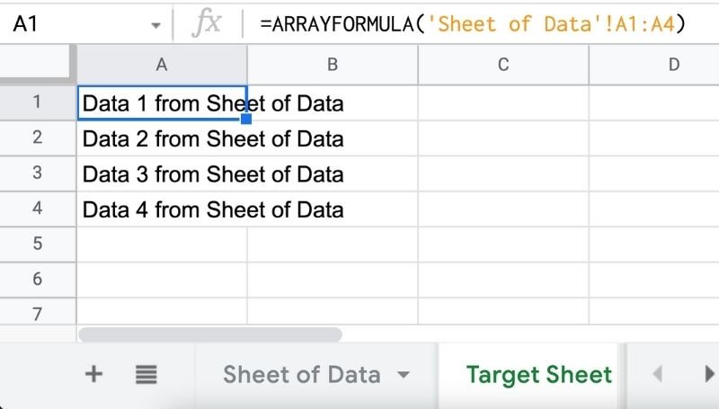
In this scenario, we will label the first tab as Data and the second one as Target. This will make things easier to understand. Data has the list of items in it and we want that same list of items to show up in our Target sheet. So, keep that in mind. Again this works on sheets within the same workspace, same file.

1. Start on your Target sheet, highlight any cell, and type in “=ARRAYFORMULA”.
2. Everything after this will be placed within parentheses.
3. Then type in the name of your sheet tab. This is that second tab you created that has the list of items/data in it. In my case, mine is named “Data”.
4. Then follow that name by typing in !
5. And finally type in the beginning cell address followed by : and ending with the last cell address. Here you get the cell address of the list of items from the Data sheet, not the Target sheet.

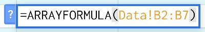
This is what your reference to a range formula should look like

After completing the simple steps above, you should have something that looks like this:

Let’s go over quickly what you’re looking at here.

The equal sign “=” is telling Google Sheets that what’s coming next is a formula.

The ARRAYFORMULA part is basically the keyword that tells Google Sheets that what you are preparing to link a set or group of data from one sheet to another.

Actually, I take that back. You “preparing to link data” is the wrong way of putting it. In fact, what ARRAYFORMULA really does is turn whatever that you key in next is not restricted to just a single value. With ARRAYFORMULA you can now add in a range. This means you’re not limited to just 1 value, you can place in a range of values by referencing the address of those values. In our case putting in one alphanumeric location and spanning everything in between up to including the last alphanumeric is acceptable in this formula or function that usually expects just one value.. I’ll explain more about this a little later on.

You’ll then need to enclose everything after this inside parentheses.

You’ll notice that the next value is called Data. That’s the name of the sheet we created that has the list of data. This tells Google Sheets that this is where all the data is coming from. This sheet called Data.

The exclamation mark “!” tells Google Sheets that this ends the name of the sheet and now it’s time to move on to the location.

The next thing Google Sheets is going to expect is where exactly the data is located. Which cells, in particular, are you referring to? Simply start with the letter and the number that correlates with the first cell which is usually located on the top left of the table or top of the column. Then place a colon in between the last cell address. In my case, it’s a single column from B2 all the way down to B7 included.

This is the range I was referring to a few paragraphs before when I was explaining what ARRAYFORMULA does. If we didn’t have it, Google Sheets would be expecting just a one cell address.

This is what you need to consider when referencing a range in Google Sheets

If you’re new to this, you’re probably scratching your head trying to understand why and what’s going on.

I find it best when I want to do something, it’s best to understand why. If you understand why and how things work, if you run into a problem, you would most likely have a better chance of fixing it. Even if you need help or research a way to fix the problem, understanding the concept will get you to a solution faster.

Check out a few of the topics below. I assure you, that you’ll need to learn these things eventually.

Sheet tabs that have 2 words as a name

I explained this pretty well in the link above in case you wanted more of an in-depth explanation.

If the name of your Data tab is made of up 2 words or more, and you followed the steps above precisely, you’ll get an error message because Google Sheets is expecting one word. Google Sheets cannot understand the spaces in between 2 separate words. And yes, that includes the spaces in between any number of words. You’ll have to find a way to tell Google that these 2 or more words should be processed as a single value. Luckily for you, the process is super simple.

In order to solve this, you can place single quotations around the full name like so:

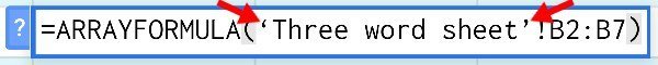
This will tell Google Sheets that it’s all one word, one name, or one value.

I know that you’re probably wondering why but this is just how it is in writing formulas. It’s called a string and sometimes when a string has multiple words in it (ie. having a space in between), you would surround that string with single quotation marks.

This is sort of the same way with how programming works. Every programmer who writes a string oftentimes surrounds that string with single quotations. At least that’s how it is in coding languages like C++.

Know how much space you need for the reference range and delegate that space only for the range needed

You probably noticed by now that referring to a list actually gets that same list to show up on the Target Sheet. Once you’ve correctly added the formula into the Target sheet and told Google this other sheet has the data and that you want Target to reference to, you’re going to notice that Target now has a copy of all your data.

By the way, this is actually not a “copy” per se. See, a copy would be a separate entity. A copy would mean that it’s separate from the original. When you alter a “copy”, this modification has no effect on the original source. That’s why I never used the word copy in this article. You are referencing the data. The target is referring to the data in the Data sheet. If you were to change the data in the data sheet, it would automatically reflect the changes in the Target sheet so be careful when editing or going back to data to change things.

Going back to the topic. You’re going to need as much empty space of as many items in the list to populate.

For example, if you plan to reference a list of 100 items in 100 cells to another target sheet. You need to make sure you have 100 sheets available for that data to fall into.

But what happens if you accidentally put something in a cell that’s already taking up space? What happens when you reference 100 items into a Target sheet with only 90 cells available? You’ll get an error. =ARRAYFORMULA won’t know what to do if there’s something blocking it from displaying the full range in that column.

It doesn’t want to overwrite data that is already there so please keep that in mind.

What if you don’t use the keyword ARRAYFORMULA in your range reference?

Not using ARRAYFORMULA will make Google Sheets think you want it to display (from the range you provided) the data that is located specifically on that numbered row that correlates with the numbered row on the Data tab.

Basically, let’s say you left out ARRAYFORMULA and had the name of the sheet along with the cell range. Either it will return in error in the realm of “this range value cannot be found” or it will try to guess what you’re trying to link which will most likely be an error.

If the address of the cell in your data list happens to match or be identical to the address of the cell you want it to display on, it will show up. An example of this is taking data from A1 on the data sheet and linking that data to A1 on another sheet, the target sheet. This will just totally create a new number you’ll probably scratch your head wondering why. But it will take the factorial of the data on that sheet which will result in a really big number.

This is all because you didn’t specify what you’re trying to do by writing in the keyword ARRAYFORMULA.

Make sure you use ARRAYFORMULA.

Add extra empty cells to your range list so you can easily add more data

There’s a way to make this list totally dynamic allowing the data you enter or will enter to continue to show up on your Target Sheet so that it can do work to it.

Here’s how.

In step 4 above when entering the last cell address, instead of putting in the last cell that has data in it, keep the cell letter but add more to the cell numbers. Here’s an example below.

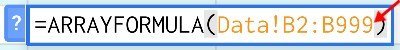
Notice how the ending address is B999 instead of B7 like it was previously? This means that I’ve pre-selected to include 999 cells in the column to fall into the rules of the formula.

From now on, whatever additional data you add in the Data column of B from 2 to 999, will show up on the Target tab as well. What this does is that it tells Google Sheets that the formula engulfs the entire column or at least all the way down to cell number 999. So anything you place within this Data column will link to the Target sheet to do work to.

Don’t worry, adding in extra empty cells won’t confuse Google Sheets. Google Sheets knows that it shouldn’t worry about empty cells until there’s something actually in it. Just a tip of caution though, if you do delegate any empty cells to the formula for future use, just be careful. Accidents can happen and you can accidentally place unrelated data in one of those cells bringing that it’s a free slot to add data to. Instead, it will show up in your target data and mess up your results.

As long as you stay organized, maybe label the columns clearly, you shouldn’t run into any trouble with this.

Conclusion

Imagine how helpful this would be if you managed several tabs that all need data from that single Data tab. I’d love to show you more of what Google Sheets can do. This is just the tip of the iceberg. Some would even argue that it’s the fundamentals. I’d say, learn this and soon, you’ll find ways to make amazing things using Google Sheets because it’s incredibly powerful as a tool for productivity.

Come back to this article anytime you like and read over the steps as much as you want. The steps will almost always stay relevant and can be incredibly helpful for any project or operation you plan to work on in the near future.